Painting the Mona Lisa using Molecular Dynamics
Recently did a project on molecular dynamics simulations for a class, and as I was doing some reading I came across this paper. While I didn’t end up reading most of it, Figure 1 stood out to me, where they set up a simulation so that the particle created a ‘density painting’ of the Mona Lisa. I thought this was very cool, and would be a great way to illustrate the concepts of ergodicity and the stationary distribution, so I set about recreating it.
The high level goal: create a simulation of a moving particle moving under a body force so that a density plot of its location history in \(\mathbb{R}^2\) paints the Mona Lisa.
The setup
The basic setup of molecular dynamics is that you have a system \(\mathcal{S}\) consisting of \(N\) particles that are immersed in a ‘reservoir’ or ‘heat bath’ \(\mathcal{R}\) containing orders of magnitude more particles than \(\mathcal{S}\). Each particle in \(\mathcal{S}\) has a position \(q\) and a momentum \(p = \dot{q}\), and combining this information for each particle into a single vector gives the state of the system \(s\) (in our case we are considering particles living in \(\mathbb{R}^2\), so \(s \in \mathbb{R}^{4N}\)). I will not write vectors in boldface just to confuse you (and because all that follows is valid also if \(q\) and \(p\) are scalars).
The combined system \(\mathcal{S} \cup \mathcal{R}\) is isolated so total energy is conserved and every possible ‘macrostate’ of this system is equally likely (this is the fundamental assumption of statistical mechanics). However, our system of interest \(\mathcal{S}\) is not isolated - it will continually exchange energy with the reservoir - so its ‘microstates’ have different probabilities of occuring. After a quick derivation (see e.g. p. 222 of (Schroeder, 2021)), the probability density of the microstates is \[ \rho(q,p) = \frac{1}{Z}\exp(-\beta H(q,p)) \] where the thermodynamic \(\beta\) is \(\beta = 1/k_B T\) and \(H(q,p) = \frac{||p||^2}{2} + U(q)\) is the total energy. This is known as the Gibbs-Boltzmann distribution.
Once we reach thermal equilibrium we expect the mean kinetic energy to be roughly constant (this is proportional to the temperature), so we can just look at the position distribution \[ \rho(q) = \frac{1}{Z}\exp(-\beta U(q)) \text{,} \] where \(U\) is a potential energy function. Thus for whatever distribution we want to sample from, as long as we can write it in the form \(\exp(-\beta U(q))\), then in theory a particle feeling the force \(F = -\nabla U\) will trace out your distribution.
Dynamics
Armed with this distribution, some 20th century boffins set out to build some stochastic differential equations (SDEs) whose solutions would be stochastic processes that sample from the distribution. What is an SDE I hear you cry? Like other differential equations, but more random.
I won’t get into the details1 but it turns out that solutions to the Langevin equations
\[\begin{align} dq &= p \,dt, \\ dp &= F(q) \, dt - \gamma p \, dt + \sqrt{2\gamma k_B T} \, dW \end{align} \] will sample the Gibbs-Boltzmann distribution.
So to sample from the distribution, i.e. simulate the movement of the particle, we discretise our equation. As an example, take \(U(q) = q^2/2\), so we would like to sample from \(\rho(q) = \exp(-q^2/2)\), which looks like this:

Our potential function \(U\) gives the force \(F = \nabla U = q\), so we numerically integrate the Langevin equations with a random initial position and velocity, and keep track of where the particle has visited (thus storing the solution’s `empirical density’). The results speak for themselves:
(or perhaps they don’t - the point is that the simulated density looks approximately like the true density function).
Great! Now all we need to do is the same thing with a different potential function.
The painting
We load in a grayscale image of the Mona Lisa:
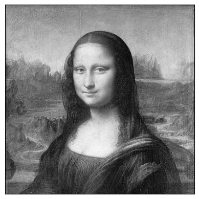
This is simply stored as a 2D array of pixel brightness, with (say) 0 for dark and 1 for light, and values in between. Let’s call the array/matrix \(A \in \mathbb{R}^{N \times N}\), where \(N\) is the number of horizontal and vertical pictures in the matrix. Now we want the particle to concentrate in the dark parts of the image and not so much in the light parts. We know that Langevin dynamics will make the particle tend towards areas of low potential, so we will think of the matrix \(A\) as encoding the values of the potential function at discrete points, i.e. \(A_{ij} = U(i,j)\), and can extend this to a definition on all of \([1,N] \times [1,N]\) by somehow interpolating between the values on this grid.
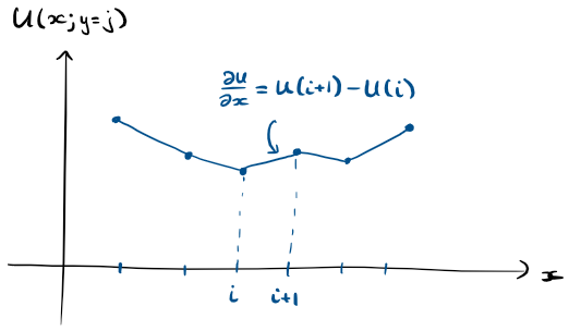
Now time for some bad (but effective) maths. In order to get our force \(F\) we need to compute \(\partial_x U\) and \(\partial_y U\). We only have concrete values for \(U\) at the discrete points \((i,j) \in \mathbb{Z} \times \mathbb{Z}\), but we can imagine that if we fixed some \(y=j\) then we’d have a one-dimensional function \(U(x;j)\) and the derivative between each of the integer points would be \(\partial U / \partial x = U(i+1) - U(i)\) (see the below figure).
Note that since \(F\) is the negative of the gradient of \(U\), we actually want \(-\partial_x U(i,j) \approx U_{i,j} - U_{i+1,j}\). How can we compute this efficiently for all appropriate \(i\) and \(j\)? Use a finite difference matrix! If \[ D := \begin{pmatrix} 1 & -1 & & & \\& 1 & -1 & & \\& & 1 & -1 &\\& & & \ddots & \ddots \end{pmatrix} \] then \(DU_{i,j} = U_{i,j} - U_{i+1,j}\), i.e. \(DU\) encodes our (negative) \(x\) derivative. Bingo! What’s more, is we can use the same matrix to get \(\partial_y U = UD\).
This gives possibly my favourite object of this project: the Mona Lisa force field
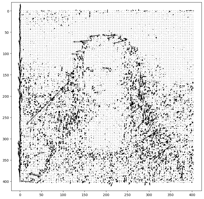
I lazily extended \(F = -\nabla U\) to a function on the full space by setting \(F(x,y) = -\nabla U_{\lfloor x \rfloor \, \lfloor y \rfloor}\).
We thus plug our Mona Lisa force field into our dynamics equations, let a particle fly about, and track where it’s been in a heatmap. We expect the heatmap (empirical density) to tend towards \(\rho(q) = \exp(-U(q))\), so to get our beloved Mona Lisa (\(U\)) back we take the log of the values in our heatmap. This gives our painting:
Now I’ll admit the results aren’t spectacular, but there is a definite Mona Lisa shaped figure being carved out. That’s good enough for me.
Afterword
I skipped a lot of details, particularly on numerical integration. You can find details of molecular dynamics simulations in Ben Leimkuhler’s book.
p.s. Adrian: the ball is in your court.
-
because I don’t know them ↩